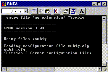
You are prompted to
give the entry filename
(here cubig, the test file) :
The model for the RMC
method is usually described with the P1 space group and the cell (generally
a cube) is large,
otherwise no acceptable
fit can be expected.
The model for the RDM method has generally to be much smaller in volume and can use space groups with any symmetry.
RMC
RMCA version 3.04 adapted for MS Windows 95/98/NT
Three files are necessary
:
cubig.dat containing
the input data
cusq.dat
the experimental structure factor
cubig.cfg
the starting model configuration
cubig.dat :
Molten copper at 1833K (example)
0.0721        ! number density
1.8           ! cut offs
0.3           ! maximum moves
0.1           ! r spacing for calculating g(r)
.false.       ! movout option
0             ! number of configurations to collect
5000          ! step for printing
100000 100000 ! step limit, step for saving
0 1 0 0       ! sets of experiments
cusq          ! file containing the experimental data
1 1000        ! first and last data point to be used
1.            ! constant to be subtracted from the data
1.            ! coefficient of each of the partial structure factors
0.01          ! standard deviation to be used
.false.       ! no renormalisation allowed
.true.        ! substract a constant from the data
0             ! the number of coordination constraints
0             ! the number of average coordination constraints
.false.       ! do not use a potential
cusq.dat
                             90   ! number of points
  Q    S(Q)
 0.1  0.032
 0.2  0.032
 0.3  0.032
 0.4  0.032
 0.5  0.033
 0.6  0.033
 0.7  0.034
 0.8  0.035
 0.9  0.037
 1.0  0.040
 1.1  0.045
 1.2  0.050
 1.3  0.056
 1.4  0.060
 1.5  0.070
 1.6  0.080
 1.7  0.092
 1.8  0.104
 1.9  0.125
 2.0  0.146
 2.1  0.186
 2.2  0.249
 2.3  0.345
 2.4  0.494
 2.5  0.717
 2.6  1.034
 2.7  1.472
 2.8  1.946
 2.9  2.333
 3.0  2.405
 3.1  2.094
 3.2  1.711
 3.3  1.412
 3.4  1.162
 3.5  0.971
 3.6  0.844
 3.7  0.763
 3.8  0.706
 3.9  0.676
 4.0  0.665
 4.1  0.659
 4.2  0.666
 4.3  0.684
 4.4  0.710
 4.5  0.747
 4.6  0.796
 4.7  0.853
 4.8  0.917
 4.9  0.982
 5.0  1.048
 5.1  1.106
 5.2  1.152
 5.3  1.184
 5.4  1.204
 5.5  1.210
 5.6  1.204
 5.7  1.191
 5.8  1.170
 5.9  1.140
 6.0  1.105
 6.1  1.066
 6.2  1.026
 6.3  0.983
 6.4  0.947
 6.5  0.917
 6.6  0.892
 6.7  0.878
 6.8  0.874
 6.9  0.877
 7.0  0.883
 7.1  0.894
 7.2  0.908
 7.3  0.928
 7.4  0.949
 7.5  0.977
 7.6  1.006
 7.7  1.030
 7.8  1.050
 7.9  1.068
 8.0  1.077
 8.1  1.083
 8.2  1.089
 8.3  1.086
 8.4  1.081
 8.5  1.074
 8.6  1.064
 8.7  1.051
 8.8  1.037
 8.9  1.022
 9.0  1.006
cubig.cfg
1000 atoms instead of 250 in the original test file
 (Version 3 format configuration file)
 Molten copper at 1833K (example)

          0         0         0 moves generated, tried, accepted
          0                     configurations saved

       1000 molecules (of all types)
          1 types of molecule
          1 is the largest number of atoms in a molecule
          0 Euler angles are provided

          F (Box is not truncated octahedral)
            Defining vectors are:
             12.013180   0.000000   0.000000
              0.000000  12.013180   0.000000
              0.000000   0.000000  12.013180

       1000 molecules of type  1
          1 atomic sites
              0.000000   0.000000   0.000000

   .9196923   .1548150  -.0943317
  -.3346117   .6183939  -.9237950
  -.4528992   .2881331  -.7544799
   .5379519  -.6989901  -.7080133
  -.9118490  -.9915042   .8107431
  -.5156245   .5272276   .4234371
   .6263573  -.4933300  -.6551015
   .8152699  -.9060440  -.4479053
  -.7255063  -.9945467   .1756687
   .4897227   .0705695  -.3118713
  -.0631945  -.4620032  -.3637259
   .0542624  -.3182621  -.8498340
  -.9211609   .5232799   .0895600
  -.7179573   .7556443   .2359407
   .4271245   .4311512  -.2984509
   .9585254   .4311182  -.7975345
  -.9864533  -.3055694   .3359582
  -.5864899  -.1665049  -.9037373
  -.5016937  -.5432656  -.5599139
  -.1678917   .9722855   .9187276
   .5893233   .8015096   .3142083
   .4247720  -.0324373   .0469940
   .8045657  -.0929770  -.4276597
   .6485779  -.9121034   .7255056
  -.3900716   .4286218   .6919811
  -.5504930  -.5362611   .6071227
  -.2769177   .1503153  -.4037516
  -.3871083  -.2395763  -.2836797
  -.9566000   .9531317   .1674922
  -.8311410  -.1360052   .3653142
   .9791048  -.5493712  -.3031456
   .5565310   .6572611  -.2218001
   .7724123   .3472662   .3798208
  -.3381078  -.9842072  -.1648724
   .9246771   .3261070  -.4739153
etc
The PC
RMCA program starts by :
a double click on its
name in the Windows Explorer,
or typing 'rmca' in a
DOS box opened in the directory containing rmca.exe and the data files.
|
You are prompted to give the entry filename (here cubig, the test file) : |
 |
The PC version shows some
minor differences with the original RMCA software :
The .his (histogram) file
is not created,
and the timelim and timesav
parameters have different significations.
Instead of being the
time the program should run for, in minutes, timelim is now the total number
of moves generated before the program will stop. Timesav is the interval
number or generated moves at which the results should be saved to the output
file.
Also the file containing the experimental data (cusq.dat here) is given without the .dat extension in the main data file (cubig.dat here).
Get the manual RMCA.ps
and the Fortran source code at the
RMCA
FTP server :
ftp://www.studsvik.uu.se/pub/rmc/rmca/
Running the test file, you should see at the end :
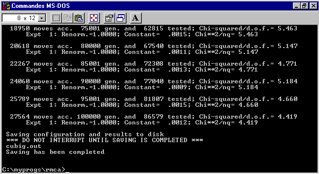
the Chi**2 oscillates
around 5 after 15000 accepted moves
LIVE DEMONSTRATION
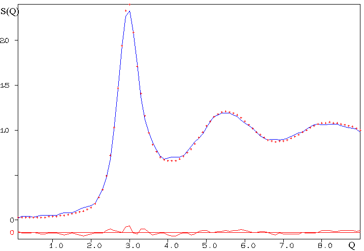
The resulting fit of S(Q)
is the following :
Some hints and tips
What is the main function
acting in RMCA :
RAN (in Fortran language)
the random number generator
used for selecting the
moving atom
as well as
for deciding of the x,y,z
moves
Why the calculation may
be so fast ?
Many elements needed for
calculating the interference function
are stored in memory
Only are recalculated
those corresponding to the moving atom
RDM
In order to apply the RDM method to glasses, one should dispose of crystalline-based starting models presenting the same composition or at least the same formulation as the material to be modelled.
The disorder is statistically introduced by microstrain effects leading to line broadening on the diffraction pattern.
The cell volume may be
adjusted for corresponding to
the measured glass density.
A preliminary test consists in looking at the starting agreement between observed and calculated S(2q) selecting some standard line broadening parameters (they can be easily adjusted by hand) and refining the scale factors.
In case of non ideal composition, for instance modelling a NaPbFe2F9 glass starting from coordinates of KCaAl2F9, after cell adaptation, the best would be to refine first the F atom coordinates, expecting adjustment of Pb-F (~2.50 Å), Na-F (~2.35 Å) and Fe-F (~1.93 Å) distances replacing respectively the K-F (~2.80 Å), Ca-F (~2.40 Å) and Al-F (~1.81 Å) ones (one should try Pb/Na permutation too and also some statistical disorder). The next step, if some convergence has been obtained, is to refine all atomic coordinates. This supposes that a maximum of independent diffraction data have been collected. Testing a model with this complexity would require the largest possible number of oscillations on diffraction data, say at least a total of 25 bumps which could correspond to 3 independent structure factors exhibiting 8 or 9 oscillations each of them. Finally, the line-broadening parameters could be refined and even the cell parameters. The process converges, or not, with agreement factors specific to the models.
Which model can we use
for molten Cu ?
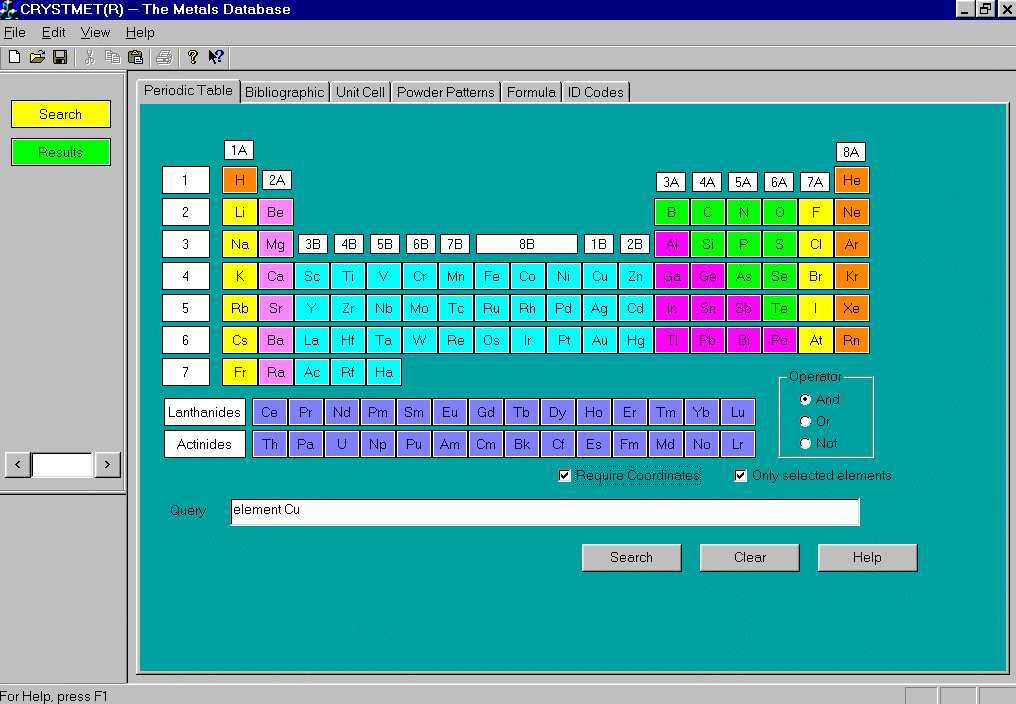
Certainly first the Cu
crystal structure
If you possess CRYSTMET,
it is readily obtained
LIVE DEMONSTRATION
Cubic Close Packed (CCP)
= face centered cubic
Fm3m
a = 3.6144 A
Cu in (4a) Wyckoff position
at x = 0, y = 0, z = 0
But, the liquid density corresponds to 0.0721 atom/Å3
and Cu solid at room temperature
has :
V = a3 = 47.22
Å3
with 4 Cu atoms per cell
:
4 / 47.22 = 0.0847
We need a cell volume
of
4 / 0.0721 =55.478 Å3
Corresponding to a = 3.8139 Å
ARITVE version 2000 for
MS Windows 95/98/NT
ARITVE is simply a Rietveld method program allowing :
- a huge limit of reflection
number (60000 on each pattern)
- 3 interference functions
maximum fitted simultaneously
- a huge limit of reflections
overlapping at the same angle (20000)
- a small number of parameters
to be refined (max = 75)
- only Gaussian peak
shape
- line broadening following
the Caglioti law
Two files are necessary :
cuCCP.dat containing
the input data
cust.nor
the experimental structure factor
cuCCP.dat :
Molten copper at 1833K  CCP        ! title
90 1 3 1 1 1 1 1 1 1               ! ncycles, npat, maxs, ng, codes
Cu                                 ! title
1                                  ! kxr (1=neutron, 4=X-ray)
1 1                                ! NA, KL
0.700                              ! Wavelength
0.05 0.1 0.8 0.05                  ! damping factors
F M 3 M                            ! Space group
0.5800                             ! scattering factor
CU                                 ! title for each atom
 1 0.0000 0.0000 0.0000 0.0400     ! ntyp, x, y, z, occup
46.7  500000. 10000. 50000.        ! scale, U, V, W
3.8139 3.8139 3.81390 90. 90. 90.  ! a, b, c, a,  b,  g
2                                  ! Nexcl (nber excluded zones)
0 300                              ! 2q1 2q2 (x100)
5600 15000                         ! 2q1 2q2 (x100)
1.0                                ! scale before refinement
cust.nor                           ! interference function filename
0 0 0 0                            ! refinement codes for x,y,z,occ
11                                 ! refinement code for scale
0 0 21                             ! refinement code for U, V, W
31 31 31 0 0 0                     ! refinement codes for cell
cust.nor
Same as cusq.dat from
RMCA, but with constant 2q
step
and x1000 (arbitrary
scale)
      119  0.00  0.50  ! number of points, starting angle, step (°2q)
   0.00000E+00   0.25066E+02   0.32000E+02   0.32000E+02   0.32133E+02
   0.32916E+02   0.33000E+02   0.33482E+02   0.34265E+02   0.35096E+02
   0.36661E+02   0.38839E+02   0.41976E+02   0.45887E+02   0.49797E+02
   0.54447E+02   0.58090E+02   0.63039E+02   0.70849E+02   0.78657E+02
   0.87753E+02   0.97115E+02   0.10833E+03   0.12470E+03   0.14106E+03
   0.16775E+03   0.20629E+03   0.25862E+03   0.33328E+03   0.44261E+03
   0.59032E+03   0.78304E+03   0.10290E+04   0.13667E+04   0.17254E+04
   0.20656E+04   0.23390E+04   0.23947E+04   0.22093E+04   0.19402E+04
   0.16592E+04   0.14286E+04   0.12333E+04   0.10694E+04   0.93876E+03
   0.84218E+03   0.77998E+03   0.73122E+03   0.69628E+03   0.67501E+03
   0.66659E+03   0.66128E+03   0.66168E+03   0.66863E+03   0.68234E+03
   0.70140E+03   0.72589E+03   0.75627E+03   0.79346E+03   0.83624E+03
   0.88263E+03   0.93124E+03   0.98034E+03   0.10301E+04   0.10760E+04
   0.11168E+04   0.11514E+04   0.11756E+04   0.11937E+04   0.12054E+04
   0.12099E+04   0.12056E+04   0.11978E+04   0.11864E+04   0.11708E+04
   0.11489E+04   0.11244E+04   0.10978E+04   0.10689E+04   0.10395E+04
   0.10088E+04   0.97815E+03   0.95172E+03   0.92894E+03   0.90865E+03
   0.89109E+03   0.88088E+03   0.87591E+03   0.87475E+03   0.87692E+03
   0.88119E+03   0.88764E+03   0.89601E+03   0.90610E+03   0.91966E+03
   0.93431E+03   0.94948E+03   0.96949E+03   0.98991E+03   0.10098E+04
   0.10268E+04   0.10415E+04   0.10551E+04   0.10678E+04   0.10743E+04
   0.10794E+04   0.10836E+04   0.10878E+04   0.10875E+04   0.10850E+04
   0.10815E+04   0.10769E+04   0.10712E+04   0.10643E+04   0.10554E+04
   0.10461E+04   0.10365E+04   0.10262E+04   0.10156E+04   0.10000E+04
The PC ARITVE
program starts by :
a double click on its
name in the Windows Explorer,
or typing 'aritve' in
a DOS box opened in the directory containing aritve.exe and the data files.
A window is opened.
You are prompted to give
the entry filename
(here cuCCP, the test
file) :
Live Demonstration
At the end of the calculation, you should have :

And the fit looks like :
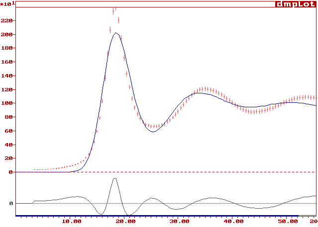
Not as good as the RMC fit, but remember the small cell containing only 4 Cu atoms. Nevertheless, similitudes are there. One can imagine that a better fit would be obtained if the model size was extended.
Combining some aspects
of both methods, is that
possible ?
Some directions to explore :
A powder diffraction pattern from the RMC result could be calculated exactly in the same way as by the RDM method.
The problem is to build a special program for the simulation of powder patterns in case of P1 space group with cell parameters of 30 Å or more.
The reflection number
for Q up to 25 Å-1
would be probably larger
than 106.
There is no serious difficulty
to code a program doing that, but this was not realized up to now.
60000 reflections maximum
are allowed per pattern, and 20000 which could overlap at a given diffracting
angle, in the present RDM ARITVE software. This is already considerable
!
Using the Rietveld method for glass modelling supposes that one accepts the idea that a selected crystal structure may represent a mean model for a glass, or a nanocrystalline material.
The disorder is statistically introduced by microstrain effect, leading to strong line broadening on the diffraction pattern.
If the mean RDM small models were physically sound, then they should be able to represent good starting configurations for RMC modelling, that would really introduce locally the disorder treated statistically in RDM modelling.
It was thus decided to enlarge some previously established RDM models, so as to build starting RMC configurations to be tested. In all cases presented hereafter, some initial coordinations were constrained during the Monte Carlo process (SiO4 and ZnCl4 tetrahedra; MF6 octahedra), so that the final RMC models were obtained from small random atom moves, keeping essentially the crystal structure features of the RDM starting models.
Which interference functions
were modelled ?
With the RMC method, the neutron and X-ray data were simulated as F(Q) data, the total coherent scattering functions (TSF) :
F(Q) = [Icoh(Q)-<f2>] / <f>2,
where the <f2>
and <f>2 terms are the usual mean diffusion factors, depending
on Q (X-ray) or not (neutron).
The RDM final models were selected among many possibilities as those providing the best Rp reliability factor.
Testing a model by the RDM method, the data fitted become :
S(2q) = Icoh(2q)/<f2>.
Q = 4psinq/l
Characterizing the fit
quality
A reliability Rp factor
was calculated as :
100*å
|Iobs-kIcalc|/å
|Iobs| (%)
(according to the definition I(Q) = F(Q)+1, k being a scale factor).