Attach the sample can to the copper block with screws that are the correct length as screws that are too long can damage the heating element or temperature sensor. Also, make sure these screws are tight, so that the screws do not loosen due to vibration.
The inner heat shield cans should not be screwed on tightly, as they may be impossible to remove after temperature cycling. Back them off by a quarter turn.
Attach the outer vacuum can and pump down with a turbopump. As soon as the
pressure is in the range of  torr, the cooling can be started. It
will typically take about 3 hours to bring the sample to
the minimum temperature.
I do not recommend attempting to collect room temperature
data with the set point at 295 K, while the displex is initially cooled as
temperature control may not be good.
When I collect data over a range of temperatures, I
tend to start at the lowest temperature first, but I cannot defend this choice
to be the best.
For runs of a day or so, one can usually operate the refrigerator without continual pumping, but cooling can fail if the pressure rises, so it is usually worth the effort to leave a pump attached while data are collected. Always use a pump with the high-temperature refrigerator, when operating above room temperature in case of outgassing.
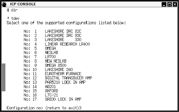
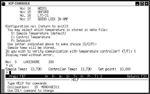
The tdev command sets the T+ flag in ICP, so that the temperature is recorded at each data point.
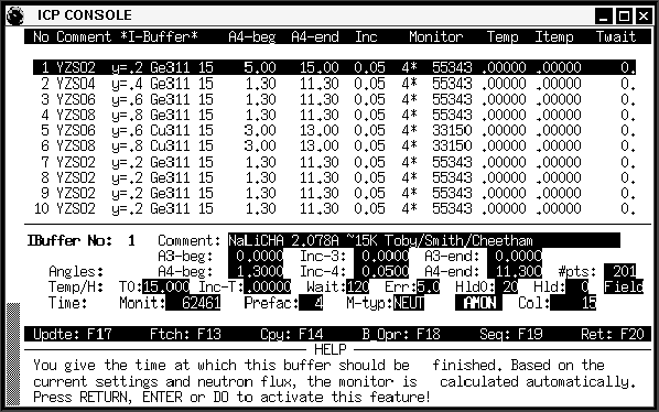
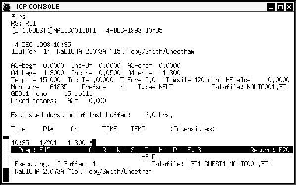
For use with a temperature controller, you will typically need to set the following fields in the buffer: Comment, T0, Wait, Err, Hld, Monit, Prefac. and M-typ, which are used as follows:
- Comment
- This sets a 1-line file header and the name of the data collection file. Be sure to use letters and numbers (A-Z and 0-9) and no other characters for the first five letters of the Comment as this is used for the file name. If an invalid name is used the file will be named DEFLTxxx.BT1, where xxx is a number in the range 001 to 999.
- T0
- This specifies the nominal temperature for data collection. This value is sent as the set point to the temperature controller. For the controllers attached to the He refrigerators, this is a temperature in K. If T0 is set to 0, and the T+ flag is set, the temperature will be recorded, but will not be changed and the Wait and Hld0 terms (below) are ignored.
- Wait
- This specifies a maximum amount of time in minutes that ICP will wait for the sample temperature to be in range (see ERR, below), before starting data collection time. If the desired sample temperature is reached in less time, the remaining time wait is not used. Typical practice is to use a wait that is much longer than the expected time needed to reach the desired temperature, for example 120 to 180 minutes. If you do not want data collection to wait for the temperature to be reached, Wait can be set to 0.
- Err
- The temperature is considered ``in range'' if the temperature is between T0+ERR and T0-ERR. Note that the value for ERR does not affect the actual stability of the temperature (which is determined by the PID parameters set in the temperature controller) so setting ERR to a small number, can cause data collection to be suspended for long periods when temperature control is flaky. Typical values for ERR are 2 to 5 K for low temperature measurements, but may be 5 to 10 K near room temperature or above.
- Hld0
- This specifies an amount of time in minutes to wait for temperature to equilibrate after the temperature is reached (or Wait expires) before data collection is started. The desired value for this parameter will depend on the experiment to be performed. A value of 20 minutes is common, but so is 0 as well as longer times.
- M-typ
- Is either ``NEUT'' or ``TIME''. NEUT is used for most data collection, where the data collection time is adjusted to match the neutron flux on the sample.
- Prefac
- Each data point is measured ``Prefac'' times and if Prefac is 4 or greater, the measurements are checked for statistical agreement, so that significant noise spikes can be discarded. A rule of thumb is that Prefac should be 4 for runs of 6 hours or less. It may be desirable to increase Prefac by 1 for each additional 6 hours of length, but 4 is a good default value regardless of the data collection time.
- Monit
- This value, along with Prefac, determines the length of the data collection period. If M-typ=TIME, this specifies a count time in seconds. Most commonly, M-typ=NEUT and Monit is set using the AUTOMON (AMON) feature.
Note that two fields, Hld and Inc-T, should always be 0. Inc-T causes the temperature to be changed for each data point and Hld creates a delay that is executed at each data point. These processes are almost never of use at BT-1.
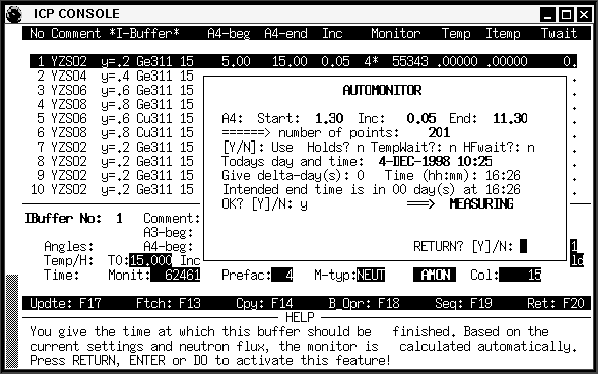
The Automon computation can either use or ignore the Wait and Hld0 values. If you answer Y for ``Use Holds,'' the time needed for the Hld0 (and Hld) hold is included in the run length computation. If you answer Y for ``Use TempWait,'' the entire Wait period is included in the run length computation. Since the entire Wait period is usually not used, it is best to say N for ``Use TempWait'' but the answer for ``Use Holds'' is a matter of personal convenience. The number of days and the end time for the run are then entered. Use 1 for delta-days if the run will go past midnight even if the run length is only a few hours. A run starting at 21:00 (9 pm) and ending at 9:00 (9 am) the next morning, would be entered as delta-days=1 and Time=9:00. The computed Monit value is set when Automon completes.
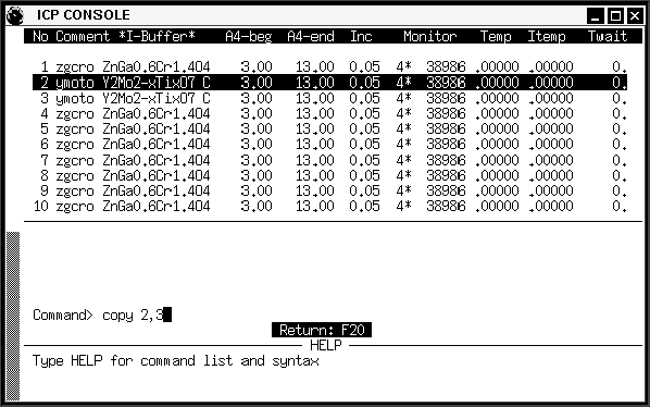
This copies the parameters in buffer #2 into buffer #3. Exit ``Buffer Ops'' mode by pressing the F20 key (actually F12). Each buffer can then be quickly modified to change the temperature (T0) and possibly the Comment, Hld0, Err and Wait values.
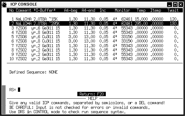
Commands are added to the run sequence by typing RI#, where
#
is the buffer number of the run in the list. Commands may be entered one a time
or several commands may be entered at once, separated by semicolons (;).
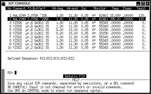
The run sequence in Figure 11 will cause buffer #1 to be collected
three times and then buffer #2 to be collected twice. Note that the files
will all be named NALICxxx.BT1, so if no other files exist, the data files
will be named NALIC001.BT1, NALIC002.BT1 and NALIC003.BT1 for 15 K runs and
NALIC004.BT1 and NALIC005.BT1 for the 295 K runs. Exit the RS menu with the
F20 key (actually F12).
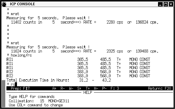
Note that the estimated lengths will be estimated assuming the maximum delay allowed by Wait and the minimum assumes that all Wait times are negligible. In the example shown in Figure 12, there are no actual temperature changes, except between the third run and the fourth, and perhaps before the first run. Assuming that the sample is already at the appropriate temperature and the refrigerator will need approximately one hour to heat from 15 K to 295 K, a good estimate is that the runs will require 32.2 hours. Your mileage may vary.
- (a)
- be sure the shutter is open
- (b)
- measure the monitor using the MRAT command
- (c)
- enter the sample composition and contact info on the white board
- (d)
- put the sample tag in the holder on the white board
- (e)
- enter the sample information in the log book (see Figure 12).
Note that it is possible to modify the run sequence or change the measurement parameters for the runs that have not been started in another (ExtraICP) window while the data collection is in progress.
If samples will be changed quickly, it may be necessary to use a heat gun to drive off condensation, but be careful not to heat the cold-head or sample stage to much more than room temperature. The refrigerator can be severely damaged by heating it above about 50 C.
